FJ Matlab Tutorial
Contents
- Vectors and Matrices
- Indexing: accessing array elements
- Reshpaing Arrays
- Plotting
- Random numbers
- Linear Equations
- Least Square Linear Regression:
- Optimization
- Nonlinear Least Square
- Numeric Root Finding
- Symbolic Root Finding
- Symbolic Calculus
- Symbolic Vector Calculus
- Symblic Ordinary Differential Equations
- Symbolic Laplace and Fourier Transforms
- Tables (dataframes)
- Data Import and File I/O
- Programming: functions, while, for, if, else, and, or, not
- Environment and Commands
- Matlab Publish, Markup and Latex
Vectors and Matrices
colon operator :
1:10
v=1:2:10
ans =
     1     2     3     4     5     6     7     8     9    10
v =
     1     3     5     7     9
Pointwise multuplication and powers of arrays: A.*B and A.^3 (A*B is -matrix- multiplication)
v_sqaured = v.^2

fprintf('norm of v = %f = %f  = %f\n', norm(v), sqrt(dot(v,v)), sum(v.^2)^.5)
v_sqaured =
     1     9    25    49    81
norm of v = 12.845233 = 12.845233  = 12.845233
linspace()
linspace(1,3,7)
ans =
    1.0000    1.3333    1.6667    2.0000    2.3333    2.6667    3.0000
Some functions: size(A), min(A), max(A), sin(A), sum(A), mean(A), isprime(A), A*A prod(A,1), A + 3, A .^2, 2*A, A+A, cross(v,w), find(A==13), union(v,w)
Other ways of creating arrays:
eye(3), zeros(3), ones(3,4), diag([1 2 3]), rand(3,4), randn(1,100), rand(3,4,2) (3-dim array)
m4=magic(4) % magic square!
sum_cols =sum(m4)  % sum of columns
sum_rows = sum(m4, 2)  % sum of rows
sum_diagnoal = sum(diag(m4))  % sum of diagonals
m4 =
    16     2     3    13
     5    11    10     8
     9     7     6    12
     4    14    15     1
sum_cols =
    34    34    34    34
sum_rows =
    34
    34
    34
    34
sum_diagnoal =
    34
A_random = randi([-3,5], 3, 7)  % a random 3*7 matrix of  integers  between -3 and 5
rank_A = rank(A_random)
A_random =
     4    -1    -2     1     2    -1     0
    -1     5    -1     0     1     3     2
     4     0     2     4     5     3    -3
rank_A =
     3
null(A): An orthornomal basis for the null space of matrix A
null_A = null(A_random)
matrix_dimensions = size(null_A)
% verify orthonormality by showing null_A' * null_A = 4*4 identity matrix
norm_of_difference = norm(null_A' * null_A - eye(4))
fprintf('verifying orthonormality, i.e., null_A'' * null_A = eye(4). In fact norm of the difference = %.15f\n', norm_of_difference)
null_A =
   -0.3241   -0.5346   -0.0018    0.1021
   -0.0680   -0.2468   -0.5029   -0.2662
   -0.3141   -0.2148   -0.3684    0.4663
    0.8593   -0.1623   -0.1263    0.1212
   -0.1816    0.7500   -0.1781    0.0953
   -0.1039   -0.1241    0.7499    0.0539
    0.0977    0.0535    0.0365    0.8213
matrix_dimensions =
     7     4
norm_of_difference =
   2.4252e-16
verifying orthonormality, i.e., null_A' * null_A = eye(4). In fact norm of the difference = 0.000000000000000
Indexing: accessing array elements
% *submatrices*
p5 = pascal(5)  % binomial coefficient
p5([1 3 5], [1  3])
p5(3:5,:)
p5 =
     1     1     1     1     1
     1     2     3     4     5
     1     3     6    10    15
     1     4    10    20    35
     1     5    15    35    70
ans =
     1     1
     1     6
     1    15
ans =
     1     3     6    10    15
     1     4    10    20    35
     1     5    15    35    70
Cholesky decomposition of a symmteric matrix: chol(A)
c = chol(p5)
is_correct = isequal(c'*c, p5)  %verify correctness of cholesky decomposition
c =
     1     1     1     1     1
     0     1     2     3     4
     0     0     1     3     6
     0     0     0     1     4
     0     0     0     0     1
is_correct =
     1
logical indexing
p5(p5 < 5)=0
p5 =
     0     0     0     0     0
     0     0     0     0     5
     0     0     6    10    15
     0     0    10    20    35
     0     5    15    35    70
indexing to new shape and end keyword
a = 1:10
a([3 4 6 8; 4 7 8 9])  % preserving shape of indexing
a(3:end)  %end key word
a(1:4:end)
a =
     1     2     3     4     5     6     7     8     9    10
ans =
     3     4     6     8
     4     7     8     9
ans =
     3     4     5     6     7     8     9    10
ans =
     1     5     9
Reshpaing Arrays
Concatenating matrices
A = ones(2,3)*5;  % 2 by 3 matrix of all 5's.
B=rand(2,3);   % 2 by 3 matrix of uniform [0,1] random numbers
C=[A;B]  % cat horizontal (B below A)
D=[A,B]  % cat vertical (B to right of A)
C =
    5.0000    5.0000    5.0000
    5.0000    5.0000    5.0000
    0.0540    0.7792    0.1299
    0.5308    0.9340    0.5688
D =
    5.0000    5.0000    5.0000    0.0540    0.7792    0.1299
    5.0000    5.0000    5.0000    0.5308    0.9340    0.5688
Deleting rows and columns
D(:, 4) = [] % deleting one column
C([2 3], :) = [] % deleting two rows
D =
    5.0000    5.0000    5.0000    0.7792    0.1299
    5.0000    5.0000    5.0000    0.9340    0.5688
C =
    5.0000    5.0000    5.0000
    0.5308    0.9340    0.5688
transpose, revel, reshape
C_transpose = C' % transpose
C_ravel = C(:)' % ravelling
C(3,6)=99  % assinging out of array bounds expand array
m4_resphape = reshape(magic(4), [2,8])  % reshaping a 4*4 matrix into a 2*8 matrix
C_transpose =
    5.0000    0.5308
    5.0000    0.9340
    5.0000    0.5688
C_ravel =
    5.0000    0.5308    5.0000    0.9340    5.0000    0.5688
C =
    5.0000    5.0000    5.0000         0         0         0
    0.5308    0.9340    0.5688         0         0         0
         0         0         0         0         0   99.0000
m4_resphape =
    16     9     2     7     3     6    13    12
     5     4    11    14    10    15     8     1
Plotting
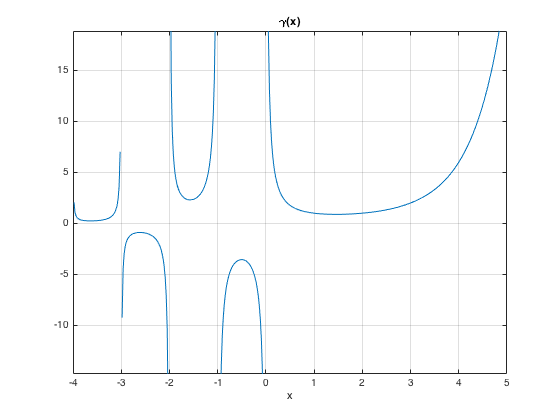
ezplot() - just give (optionally) the range (usally as [a,b]). Has symbolic version too: syms x y; ezplot(x^2)
ezplot('gamma(x)',[-4,5]), grid on % gamma function: has ploes at 0 and negative integers
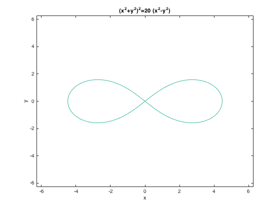
ezplot('(x^2+y^2)^2=20*(x^2-y^2)') % implicit
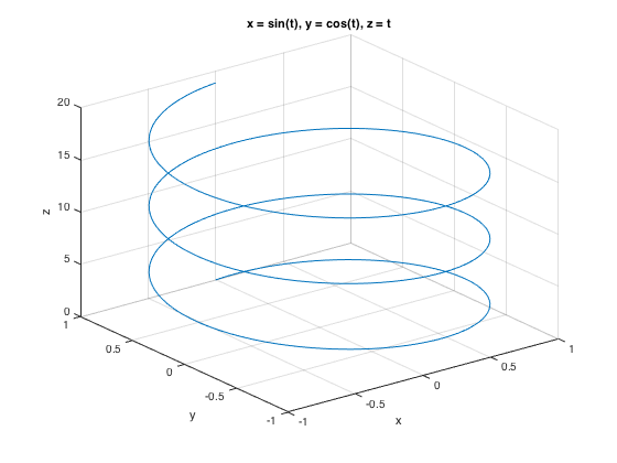
parametric 3D: ezplot3() (ezplot() does 2D parametrix), e.g., ezplot('cos(3*t)', 'sin(2*t)')
ezplot3('sin(t)','cos(t)','t',[0,6*pi])
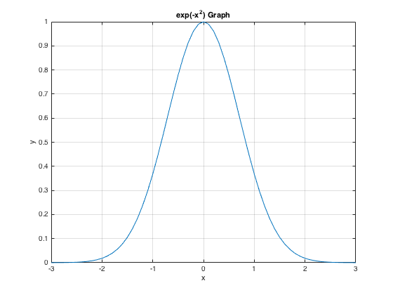
x-y plotting: plot() (also fplot())
x = -3:.1:3;
y = exp(-x.^2);
plot(x,y)
grid on, xlabel('x'), ylabel('y'), title('exp(-x^2) Graph')
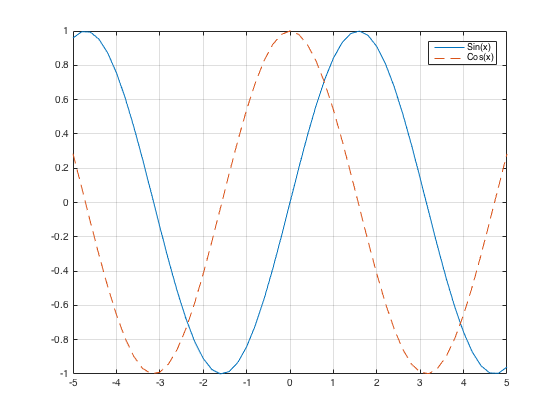
Plotting two curves Either use "hold on" or plot(x,y1,x,y2)
x = -5:.2:5;
plot(x, sin(x), x, cos(x), '--'), legend('Sin(x)', 'Cos(x)'), grid on
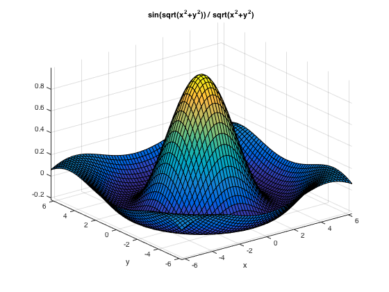
Surface plot: ezsurf() or ezsurfc() to also see the contours
ezsurf('sin(sqrt(x^2+y^2)) / sqrt(x^2+y^2)') % may use a different domain , e.g. [-7,7] (applicable to both x y), or [-7,7,-4,4]
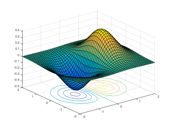
Surface plot: surf() or surfc() to also see the contours
[x,y] = meshgrid(-2:.1:2);
g = x .* exp(-x.^2 - y.^2);
surfc(x, y, g)
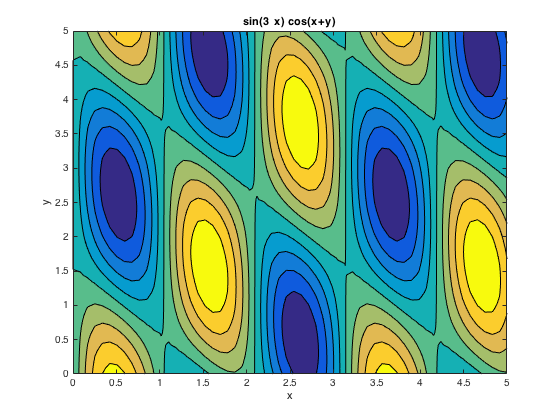
Contour plot: ezcontourf()
ezcontourf('sin(3*x)*cos(x+y)',[0,5])
% colormap('spring')  % changing color
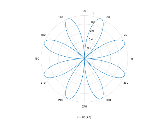
Polar coordinatee: polar() or simply ezpolar('sin(4*t)')
ezpolar('sin(4*t)')

%t = 0:0.01:2*pi;
%r = sin(4*t);
%polar(t, r, 'red')  % this renders in red
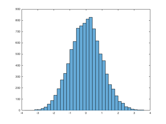
Histogram: histogram()
x = randn(10000,1);  %10000 random normals
histogram(x)
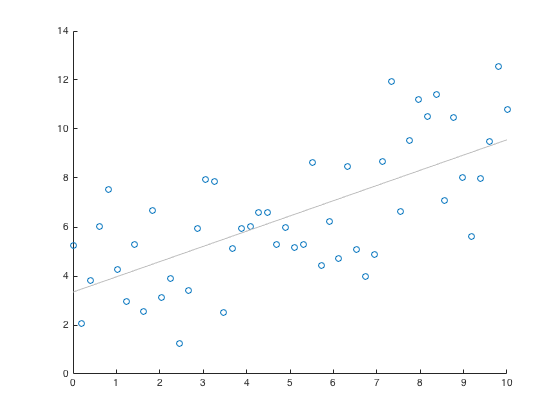
Scatter Plot : scatter()
x = linspace(0,10, 50);
y = 4 + x/2 + 2*randn(1,50);
scatter(x,y), lsline
Random numbers
First, initialize the random number generator to make the results in this example repeatable.
rng(0,'twister') % reset the seed

r_uniform = rand(1,6)  % unifrom [0,1]

r_integers = randi(12,2,9) % 2 by 9 matrix of random integer between 1 and 12

r_normal = randn(1,6)  % normal

mean_std = [mean(r_normal), std(r_normal)]  % mean and std

r_permutation = randperm(15,10)  % a length 10 random permuation of 15 element
r_uniform =
    0.8147    0.9058    0.1270    0.9134    0.6324    0.0975
r_integers =
     4    12     2    12    10     6    10     8    11
     7    12    12     6     2    11    12     1    12
r_normal =
    0.4889    1.0347    0.7269   -0.3034    0.2939   -0.7873
mean_std =
    0.2423    0.6759
r_permutation =
     9     6    10    12     3    13     4    15    11     2
Linear Equations
matrix multipication, det(), etc.
pointwise_add = [2 3 -2] +  [4 5 7]  %pointwise multplication (for vectors, matrices (all arrays))
pointwise_mult = [2 3 -2] .* [4 5 7]  %pointwise multplication (for vectors, matrices (all arrays))
A = magic(3);
matrix_multp = A * A  % = A^2, matrix multiplication
det_A = det(A) % similarly trace(A)
pointwise_add =
     6     8     5
pointwise_mult =
     8    15   -14
matrix_multp =
    91    67    67
    67    91    67
    67    67    91
det_A =
  -360
inverse and solution
inverse = inv(A) % inverse
x = linsolve(A,[1 0 0]')  %linear solve
x= A \ [1, 0, 0]'  % same linear solve, but shorter
inverse =
    0.1472   -0.1444    0.0639
   -0.0611    0.0222    0.1056
   -0.0194    0.1889   -0.1028
x =
    0.1472
   -0.0611
   -0.0194
x =
    0.1472
   -0.0611
   -0.0194
eigen values and eignen vectors
eigenvalues = eig(A) % eigenvalues
[V,D] = eig(A)  % eigen vectors and eigen values
eigenvalues =
   15.0000
    4.8990
   -4.8990
V =
   -0.5774   -0.8131   -0.3416
   -0.5774    0.4714   -0.4714
   -0.5774    0.3416    0.8131
D =
   15.0000         0         0
         0    4.8990         0
         0         0   -4.8990
Least Square Linear Regression:
short way using X \y
x1 = [.2 .5 .6 .8 1.0 1.1]';
x2 = [.1 .3 .4 .9 1.1 1.4]';
X = [ones(size(x1)) x1 x2];
y = [.17 .26 .28 .23 .27 .34]';
b = X \ y
b =
    0.1203
    0.3284
   -0.1312
long way using lscov(X,y). But can also return standard error of coefficients amd mean square error
[b,se_b,mse] = lscov(X,y)
b =
    0.1203
    0.3284
   -0.1312
se_b =
    0.0643
    0.2267
    0.1488
mse =
    0.0015
polynomial curve fitting
x = [1 2 3 4 5 6]; y = [5.5 43.1 128 290.7 498.4 978.67]; %data
p = polyfit(x,y,4) % ax^4 + bx^2 + . . .
response_vs_fitted = [y;polyval(p,x)]
p =
    4.1056  -47.9607  222.2598 -362.7453  191.1250
response_vs_fitted =
    5.5000   43.1000  128.0000  290.7000  498.4000  978.6700
    6.7844   36.6780  140.8440  277.8560  504.8220  977.3856
Optimization
For maximizing f(x), minimize -f(x)
one variable: fminbnd(). Can further use
opts = optimset('Display','iter');
To find the minimum of the humps function in the range (0.3,1), use pointer to function @humps
x = fminbnd(@humps,0.3,1) % @humps is pointer to the humps(x) funtion
x =
    0.6370
several variables: fminsearch() Find a minimum for "three_var()" function using x = -0.6, y = -1.2, z = 0.135 as starting values.
v = [-0.6 -1.2 0.135]; %initial search
fun = @(v) v(1).^2 + 2.5*sin(v(2)) - v(3)^2*v(1)^2*v(2)^2;
fminsearch(fun, v)
%fminsearch(@three_var, v)  % here three_var() is defined in an m file
ans =
    0.0000   -1.5708    0.1803
Nonlinear Least Square
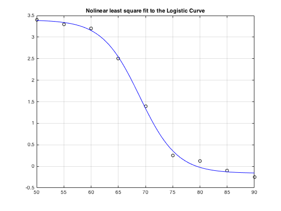
lsqcurvefit(): from Optimization toolbox. Below solving a Phyical BioChem problem
xdata = [50,55,60,65,70,75,80,85,90];
ydata = [3.4,3.3,3.2,2.5,1.4,.25,.12,-0.1,-0.25];
logistic_fun = @(x,xdata)(x(1)-x(2))./(1+exp(x(3)*(xdata-x(4)))) + x(2);
x0 = [3.5,-0.3,0.25, 69.2];
options = optimoptions('lsqcurvefit','Display','none');  % so as to suppress warning output
x = lsqcurvefit(logistic_fun,x0,xdata,ydata, [], [], options)   % x = lsqcurvefit(fun,x0,xdata,ydata)
times = linspace(xdata(1),xdata(end));
plot(xdata,ydata,'ko',times,logistic_fun(x,times),'b-')
grid on, title('Nolinear least square fit to the Logistic Curve')
x =
    3.4006   -0.1609    0.2908   68.9322
Numeric Root Finding
Numeric one equation in one unknown: fzero()
fzero() admits an interval or point as initial search, and has options
Calculate  by finding the zero of the sine function near 3.
fun = @sin; % function
x0 = 3; % initial point
x = fzero(fun,x0)
x =
    3.1416
Find the zero of cosine between 1 and 2.
fun = @cos; % function
x0 = [1 2]; % initial interval
[x,fval,exitflag,output] = fzero(fun,x0)
x =
    1.5708
fval =
   6.1232e-17
exitflag =
     1
output =
    intervaliterations: 0
            iterations: 5
             funcCount: 7
             algorithm: 'bisection, interpolation'
               message: 'Zero found in the interval [1, 2]'
root of polynomials root()
roots([1 0 -2 -5]) % x^3 -2x -5
ans =
   2.0946 + 0.0000i
  -1.0473 + 1.1359i
  -1.0473 - 1.1359i
root of function with parameter
myfun = @(x,c) cos(c*x);  % parameterized function
c = 2;                    % parameter
fun = @(x) myfun(x,c);    % function of x alone
x = fzero(fun, 0.1)
x =
    0.7854
numeric multivariable: fsolve() of Optimization Toolbox. Pass initial guess
root2d=@(x)[ exp(-exp(-x(1)+x(2))) - x(2)*(1+x(1)^2), x(1)*cos(x(2)) + x(2)*sin(x(1)) - 0.5];
x = fsolve(root2d, [0,0])
Equation solved.

fsolve completed because the vector of function values is near zero
as measured by the default value of the function tolerance, and
the problem appears regular as measured by the gradient.


x =
    0.3931    0.3366
To supress warning output, call fsolve() with option:
options = optimoptions('fsolve','Display','none');
x = fsolve(root2d, [0,0], options)
x =
    0.3931    0.3366
Symbolic Root Finding
Symbolic one equation in one unknown: solve()
syms a b c x
sol = solve(a*x^2 + b*x + c == 0) % implicity x is assumed as unknown
sola = solve(a*x^2 + b*x + c == 0, a)
Warning: The solutions are valid under the following conditions: (b + (b^2 -
4*a*c)^(1/2))/a < 0;
(b - (b^2 - 4*a*c)^(1/2))/a < 0.
 To include parameters and conditions in the solution, specify the
 'ReturnConditions' option.
sol =
 -(b + (b^2 - 4*a*c)^(1/2))/(2*a)
 -(b - (b^2 - 4*a*c)^(1/2))/(2*a)
sola =
-(c + b*x)/x^2
Symbolic numeric one equation in one unknown: vpasolve()
syms x
vpasolve(200*sin(x) == x^3 - 1, x)

vpasolve(200*sin(x) == x^3 - 1, x, 4) % with initial value 4

vpasolve(200*sin(x) == x^3 - 1, x, [-5,-3])  % in interval [-4,-3]
ans =
-0.0050000214585835715725440675982988
ans =
3.0098746383859522384063444361906
ans =
-3.0009954677086430679926572924945
Symbolic two equations in two unknowns: solve()
syms u v
[u,v]=solve([2*u^2 + v^2 == 1, u - 2*v == 0], [u, v])  % 2 dimensional
u =
 -2/3
  2/3
v =
 -1/3
  1/3
Symbolic numeric two equations in two unknowns: vpasolve()
syms x y
[sol_x, sol_y] = vpasolve([x*sin(10*x) == y^3, y^2 == exp(-2*x/3)], [x, y])
sol_x =
88.90707209659114864849280774681
sol_y =
0.00000000000013470479710676694388973703681918
Symbolic Calculus
limit
syms x
a = limit((1-cos(x))/x^2, 0)  %limit

b = limit(abs(x)/x, x, 0, 'right')
a =
1/2
b =
1
series
syms k n x
S1 = symsum(k^2, k, 0, n)  % finite sum
S2 = symsum(1/k^2, k, 1, Inf)  % infinite series
S3 = symsum(x^k,k,0,Inf)  % geomtric series
S1 =
(n*(2*n + 1)*(n + 1))/6
S2 =
pi^2/6
S3 =
piecewise([x < 1, -1/(x - 1)], [1 <= x, Inf])
derivative
syms t
f = 3*t^2 + 2*t^(-2);
diff(f)  % derivative
diff(f,2)  % second derivative
ans =
6*t - 4/t^3
ans =
12/t^4 + 6
integral
syms t
f = 3*t^2 + 2*t^(-2);
int(f)  % integral
int(f,1,2)  % definite integral
ans =
(t^4 - 2)/t
ans =
8
numerical integration

fun = @(x) exp(-x.^2).*log(x).^2;
integral(fun,0,Inf)
ans =
    1.9475
algebra
syms x y
expand(cos(x+y))
factor(x^3 - y^3)
simplify((x^4-16)/(x^2-4))
ans =
cos(x)*cos(y) - sin(x)*sin(y)
ans =
[ x - y, x^2 + x*y + y^2]
ans =
x^2 + 4
Symbolic Vector Calculus
curl(F) of a vector field F.
syms x y z
F = [x^3*y^2*z, y^3*z^2*x, z^3*x^2*y];
curl_F = curl(F, [x, y, z])
curl_F =
   x^2*z^3 - 2*x*y^3*z
   x^3*y^2 - 2*x*y*z^3
 - 2*x^3*y*z + y^3*z^2
potential function for a conservative vector field F : given F with curl(F)=0 find function f with grad(f) = F
syms x y z F f
F = [x; y; z*exp(z)]
curl_F = curl(F)' % verify cur(F) = 0
f = potential(F, [x y z])
grad_f_minus_F = simplify(gradient(f)-F)'  % verify grad f = F
F =
        x
        y
 z*exp(z)
curl_F =
[ 0, 0, 0]
f =
x^2/2 + y^2/2 + exp(z)*(z - 1)
grad_f_minus_F =
[ 0, 0, 0]
potential vector field for an incompressible vector field F: given F with div(F)=0, find P with curl(P) = F
syms x y z F P
F = [2*y^3 - 4*x*y;  2*y^2 - 16*z^2+18;  -32*x^2 - 16*x*y^2];
div_F = divergence(F)   % verfiry div(F)=0
P = vectorPotential(F, [x y z])  % solve for the potential P
curl_P_minus_F = simplify(curl(P)-F)'  % verify curl(P) = F
div_F =
0
P =
 z*(2*y^2 + 18) - (16*z^3)/3 + (16*x*y*(y^2 + 6*x))/3
                                  2*y*z*(- y^2 + 2*x)
                                                    0
curl_P_minus_F =
[ 0, 0, 0]
Laplacian: same as grad(div(f))
syms x y z
f(x,y,z)=1/sqrt(x^2+y^2+z^2)
L = laplacian(f, [x y z]);  % In the sense of generalized functions, L is the Dirac delta function at the origin
L_f = simplify(L)
f(x, y, z) =
1/(x^2 + y^2 + z^2)^(1/2)
L_f(x, y, z) =
0
Symblic Ordinary Differential Equations
First order ODE: linear, variable coefficient, homogenous
s = dsolve('Dy = 5*t*y')
s = dsolve('Dy = 5*t*y', 'y(0)=3')
s =
C5*exp((5*t^2)/2)
s =
3*exp((5*t^2)/2)
First order ODE: nonlinear,
s=dsolve('(Dy+y)^2 == 1')
% alternative syntax
syms x(t)
x(t) = dsolve((diff(x,t) + x)^2 == 1, x(0) == 0)
s =
 C10*exp(-t) + 1
 C11*exp(-t) - 1
x(t) =
 exp(-t) - 1
 1 - exp(-t)
Second order ODE: linear constant coefficient, homogenous
s = dsolve('D2y - y = 0', 'y(0) = -1', 'Dy(0) = 2')
s =
exp(t)/2 - (3*exp(-t))/2
Second order ODE: linear, inhomogenous
s=dsolve('D2y = cos(2*t) - y', 'y(0) = 1', 'Dy(0) = 0');
simplify(s)
% alternative syntax
syms y(x)
Dy = diff(y);
y(x) = dsolve(diff(y, x, x) == cos(2*x) - y, y(0) == 1, Dy(0) == 0);
y(x) = simplify(y)
ans =
1 - (8*sin(t/2)^4)/3
y(x) =
1 - (8*sin(x/2)^4)/3
Third order ODE: linear, homogenous
syms u(x)
Du = diff(u, x);
D2u = diff(u, x, 2);
u(x) = dsolve(diff(u, x, 3) == u, u(0) == 1, Du(0) == -1, D2u(0) == pi)
u(x) =
(pi*exp(x))/3 - exp(-x/2)*cos((3^(1/2)*x)/2)*(pi/3 - 1) - (3^(1/2)*exp(-x/2)*sin((3^(1/2)*x)/2)*(pi + 1))/3
System of ODE
syms f(t) g(t)
[fSol(t) gSol(t)] = dsolve(diff(f) == 3*f + 4*g, diff(g) == -4*f + 3*g)
% with initial condition:
[fSol0(t) gSol0(t)] = dsolve(diff(f) == 3*f + 4*g, diff(g) == -4*f + 3*g, f(0) == 0, g(0)==1)
fSol(t) =
C23*cos(4*t)*exp(3*t) + C22*sin(4*t)*exp(3*t)
gSol(t) =
C22*cos(4*t)*exp(3*t) - C23*sin(4*t)*exp(3*t)
fSol0(t) =
sin(4*t)*exp(3*t)
gSol0(t) =
cos(4*t)*exp(3*t)
System of ODE using matrix form
syms x(t) y(t)
A = [1 2; -1 1];
B = [1; t];
Y = [x; y];
eqn = diff(Y) == A*Y + B
[xSol(t) ySol(t)] = dsolve(eqn);
xSol(t) = simplify(xSol(t))
ySol(t) = simplify(ySol(t))
eqn(t) =
 diff(x(t), t) == x(t) + 2*y(t) + 1
   diff(y(t), t) == t - x(t) + y(t)
xSol(t) =
(2*t)/3 + 2^(1/2)*C27*exp(t)*cos(2^(1/2)*t) + 2^(1/2)*C26*exp(t)*sin(2^(1/2)*t) + 1/9
ySol(t) =
C26*exp(t)*cos(2^(1/2)*t) - t/3 - C27*exp(t)*sin(2^(1/2)*t) - 2/9
Symbolic Laplace and Fourier Transforms
Laplace transform
syms s t a b
laplace(t^9)
laplace(exp(-b*t))
laplace(sin(a*t))
ans =
362880/s^10
ans =
1/(b + s)
ans =
a/(a^2 + s^2)
inverse Laplace transform
ilaplace(1/s^7)
ilaplace(a/(s^2 + a^2))
ilaplace(s^2/(s^2 + a^2))
ans =
t^6/720
ans =
sin(a*t)
ans =
dirac(t) - a*sin(a*t)
Fourier and inverse Transforms
syms x w
f = exp(-2*x^2); %our function
FT = fourier(f) % Fourier transform
f = ifourier(-2*exp(-abs(w))) % inversre Fourier transform
FT =
(2^(1/2)*pi^(1/2)*exp(-w^2/8))/2
f =
-2/(pi*(x^2 + 1))
Tables (dataframes)
Tables are equivalent of R dataframes for data analysis
LastName = {'Smith';'Johnson';'Williams';'Jones'; 'James'};
Age = [38;43;38;40; 63];
Height = [71;69;64;67;70];
Weight = [176;163;131;133; 190];
BloodPressure = [124 93; 109 77; 125 83; 117 75; 132 85];
T = table(Age,Height,Weight,BloodPressure,...
    'RowNames',LastName)
T =
                Age    Height    Weight    BloodPressure
                ___    ______    ______    _____________
    Smith       38     71        176       124     93
    Johnson     43     69        163       109     77
    Williams    38     64        131       125     83
    Jones       40     67        133       117     75
    James       63     70        190       132     85
writetable(), readtable() read and write tables to files with choce delimter, header, etc.
% *Accessing data*
T([ 2 3],:)  % as table
T{[2 3],:}  % as data (matrix)
T.Height % or T.(2)
T(T.Age>38,:)
ans =
                Age    Height    Weight    BloodPressure
                ___    ______    ______    _____________
    Johnson     43     69        163       109     77
    Williams    38     64        131       125     83
ans =
    43    69   163   109    77
    38    64   131   125    83
ans =
    71
    69
    64
    67
    70
ans =
               Age    Height    Weight    BloodPressure
               ___    ______    ______    _____________
    Johnson    43     69        163       109     77
    Jones      40     67        133       117     75
    James      63     70        190       132     85
Data Import and File I/O
Writing numerial array to file: dlmwrite(). Reading: dlmread()
dlmwrite('magic5.txt', magic(5), ' ');
m5=dlmread('magic5.txt') % or m5=importdata('magic5.txt').
m5 =
    17    24     1     8    15
    23     5     7    14    16
     4     6    13    20    22
    10    12    19    21     3
    11    18    25     2     9
Has low level file IO similar to C
Writing a file by fopen(,'w')
x = 0:.5:3;
y = [x; log(x); exp(x)];
fid = fopen('logtable.txt', 'w');
fprintf(fid, 'x log_x exp_x\n');
fprintf(fid, '%f %f %f\n', y);  % two values appear on each row of the file, i.e., print the transpose
fclose(fid);
type logtable.txt  %display the file created
x log_x exp_x
0.000000 -Inf 1.000000
0.500000 -0.693147 1.648721
1.000000 0.000000 2.718282
1.500000 0.405465 4.481689
2.000000 0.693147 7.389056
2.500000 0.916291 12.182494
3.000000 1.098612 20.085537
Reading a file by fopen(,'r')
fid = fopen('logtable.txt', 'r');
header = fscanf(fid, '%s', 3)
line1 = fscanf(fid, '%f ', 3)'
line2 = fscanf(fid, '%f ', 3)'
fclose(fid);
header =
xlog_xexp_x
line1 =
     0  -Inf     1
line2 =
    0.5000   -0.6931    1.6487
Importing data into a table: readtable()
t = readtable('logtable.txt', 'delimiter', 'space')
t =
     x      log_x      exp_x
    ___    ________    ______
      0        -Inf         1
    0.5    -0.69315    1.6487
      1           0    2.7183
    1.5     0.40547    4.4817
      2     0.69315    7.3891
    2.5     0.91629    12.182
      3      1.0986    20.086
Importing data into a structure: importdata()
delimiter = ' ';
headers = 1;
s = importdata('logtable.txt') % or s = importdata('logtable.txt', delimiter, headers)
data = s.data
s =
          data: [7x3 double]
      textdata: {'x'  'log_x'  'exp_x'}
    colheaders: {'x'  'log_x'  'exp_x'}
data =
         0      -Inf    1.0000
    0.5000   -0.6931    1.6487
    1.0000         0    2.7183
    1.5000    0.4055    4.4817
    2.0000    0.6931    7.3891
    2.5000    0.9163   12.1825
    3.0000    1.0986   20.0855
To copy data from clipboard to A use '-pastespecial':
A = importdata('-pastespecial')
array2table(A), table2array(), summary(), size(), T.Properties.VariableNames, T.Age=[], T(1,:)=[]
Programming: functions, while, for, if, else, and, or, not
anonymous function. Can be passed as pointer to function in fzero(), etc
power = @(x, n) x.^n;
power([1 2 3],3)
ans =
     1     8    27
.m file scripts can contain anonymous function defintions, but not .m-file function defintions (neither can the interactive shell)
.m file functions can contain sub functions or nested functions but only first function is seen from outside.
An .m file function can return one or several values
function F = root2d(x)
    F(1) = exp(-exp(-x(1)+x(2))) - x(2)*(1+x(1)^2);
    F(2) = x(1)*cos(x(2)) + x(2)*sin(x(1)) - 0.5;
 end % returns a vector F
function [x1,x2] = quadratic(a,b,c)
    d = disc(a,b,c);
    x1 = (-b + d) / (2*a);
    x2 = (-b - d) / (2*a);
end % end of quadratic
function dis = disc(a,b,c)
    dis = sqrt(b^2 - 4*a*c);
end % end of sub-function
if, else (and, or)
a = 100;
if a == 10 || a == 5
    fprintf('Value of a is 10 or 5\n' );
elseif ( a == 20 && a ~= 30)
    fprintf('Value of a is 20\n' );
else
    fprintf('None of the values are matching\n');
    fprintf('Exact value of a is: %d\n', a );
end
None of the values are matching
Exact value of a is: 100
while loop
a = 10;
while( a < 13 )
    fprintf('value of a: %d\n', a);
    a = a + 1;
end
value of a: 10
value of a: 11
value of a: 12
for loop (C style)
for a = 18:-2:14
    disp(a)
end
    18
    16
    14
for loop (Python style)
for a = [24,18,17,23]
    disp(a-10)
end
    14
     8
     7
    13
Environment and Commands
semicolon: suppresses output
Continuation use an ellipsis . . ., to continue the input on the next line.
Stop execution: press Ctrl+C or Ctrl+Break. on Mac, you can also use Command+. (Command key and the period key).
Intellisense: To see the parameter list of a function, pause after typing "(".
code completition: type part of variable and press tab
clear x
clear x*    % clear all variables starting with x
clearvars x y z
clc  % clears screan
help fzero
format, format(long)  %  number of decimal digit display
quit  % quit Matlab session
who   % list of variables
pwd  % current directroy
path  % matlab path of directories
x=input('enter a number:  ')  % waits for an input
type 'filename.txt'  % displays file content
Matlab Publish, Markup and Latex
Matlab Publish
Can save notebook as html or pdf (choose Publis/Edit Publishing Options/output file format.
Unfortuantely was not able to run Matlab from Jupyter notebook - probably due to lack of Matlab support for Python 3.6.
So here I use Matlab's Publish utility (on the Publish tab of the main Matlab screen).
MatLab Markup
The first heading appears as notebook title, subsequent headings in table of contents.
Number of spaces after % determines format: 0=comment, 1=normal font, 2 =preformatted, 3=code.
This is hyperlink: MathWorks , ITALIC TEXT , BOLD TEXT, MONOSPACED TEXT. Has bullet, image, etc too.
for x = 1:10
    disp(x)  % CODE TEXT
end
Matlab Latex
Maltlab embeds (somewhat blurred) images of latex equations. Morover inline eqautions like  don't line up well.