Fitting Exponential Decay

Exponential decay is a very common process. In this week's lab we will generate some data that should follow this law, and you will have to fit exponential data at least twice more this quarter. The purpose of this lab description is to remind you how to do so.

An exponential decay curve fits the following equation: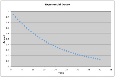

y = e ^-t/τ

. The graph of the function looks like this:

However, it is very hard for the human eye (and brain) to see how well data fall upon an exponential curve. On the other hand, humans are attuned to straight lines. The results become clearer if we take the natural log of both sides:

ln(y) = - (1/τ) t

In other words, the negative inverse of the slope will be the time constant of decay. Note that bad things happen when you take the natural log of zero, so recognize this when you are attempting your fit.

Note that often this is written in an alternate form:

y = e ^{-λ t}

and ln(y) = - λ t

Finally, the halflife of the decay is related to the decay constants in the following way:

t_1/2 = ln(2) τ = ln(2) / λ

Of course, some students need a reminder on how to do a linear fit...

Go to a computer and open Microsoft Excel. Put in your data and have Excel perform the natural log. We will next want to make a graph. Select the proper columns and then pick the Chart Wizard option from the taskbar. The button looks like this:

Pick X-Y Scatter Plot and take the default option. Add a title, labels and units to your chart. Click finish and Excel will generate a graph.

Under the Chart menu, click on "Add Trendline". Under options, display the equation and the R-squared value. This will put a least-squares fit on the graph and give the slope. The R-squared number should be close to one. If it is not, it means that some of the data may be non-linear. Note that if R-squared is equal to one, this often is a sign that you have made some kind of error as it implies straight-line data with no "noise".

Now that the slope isknown, what's the uncertainty in that slope? Excel can tell us with the LINEST feature. Go to an empty cell in Excel and type

=LINEST(known Y value cells, known X value cells, 1, true)

where "known Y value cells" are the data entries that correspond to the Ys and "known X value cells" are the Xs. For example, if we had column A as X and column B as Y, and we had eight rows of data, we would type the following:

=LINEST(B1:B8, A1:A8, 1, true)

When we type this in Excel will return a single value, the slope. LINEST is an array function, which means that even though it is trying to give back a lot of values, it only displays one per cell. What Excel is expecting you to do is highlight a 2x2 set of cells with the LINEST formula in the upper-left cell. Once this is done, go up to the formula bar and highlight the entire LINEST equation you typed in and hit Ctrl-Shirt-Enter (on a Mac use Apple-Return). This will fill in the 2x2 square. Upper left will be the slope, lower left will be the error on the slope. Upper right will be the intercept and lower right will be the error on the intercept. Make sure you remember how to get the error on your slope, as you will need to do this in almost every lab. Failure to provide error bars on your measurements is the fastest way to lose points in this class.